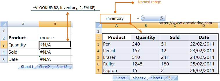
See the image. It shows how multiple Vlookup functions have failed to find the values and throws #N/A errors.

The Vlookup's threw errors because the product mouse is not listed in the table data in Sheet2.
The error #N/A actually explains nothing except that there is an error. Using the IFERROR function, we can handle these errors and show an error message-using words that are easy understand (or simply leave the cell blank) and will pinpoint the cause of the error.
Trap #N/A errors in VLOOKUP formula using IFERROR and show Empty Text
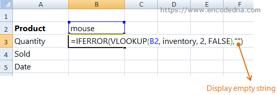
Now, let's see how you can use IFERROR function to wrap your VLOOKUP formula and if there's an error, will show a blank text (or an empty text) in the cell.
First, see the syntax.
IFERROR(value, value_if_error)
The Iferror function takes two parameters. The first parameter is the value that you want check (in our case the Vlookup formula) and the second parameter takes a value (a text, multiple words, numbers or simply an empty text), which you want to show if there is an error. Both parameters are required, that is, you cannot omit either of it.

The other rows (for Sold and Date) will have the same formula (except the columns numbers).

Trap #N/A errors in VLOOKUP formula and Show your own Text
You can show a custom message of your own like a text message (a meaningful word or two) instead of a blank text or number values like zero etc., to describe the error. For example, if the product is not the list, instead of an error, show a message like Product not found or simply a 0. See the image.

Note: Don't jumble your formula with too many or unnecessary error handlers using the IFERROR function. It can make the formula execution slow and it would hard find and fix if you are using multiple IFERROR’s in your formula. Use it judiciously.
