One of most common ways to calculate alphanumeric values in Excel are by formatting the cells value and then do the calculations, or by replacing the alphabets with a blank value and so on.
You can also use a simple formula. The formula that I am going to show you here uses a built-in function in Excel called SUBSTITUTE().
Let’s see the syntax.
Syntax of SUBSTITUTE() Function
SUBSTITUTE (text, old_text, new_text, instance_num)

It substitutes or replaces the old text with a new text in a text string. It takes four parameters.
text: a text or the cell reference whose values need to be replaced. Required.
old_text: the text that will be replaced by a new text or value. Required.
new_text: the text that will replace the old text. Required.
instance_num: This is optional. It specifies which occurrence of the old text will be replaced with new text.
Multiply Cells with Alphanumeric Values using SUBSTITUTE()
Now, let’s see how we can multiply alphanumeric values in two different cells. I have values in Cells B2 and C2.
= SUBSTITUTE(B2, "Kg", "") * SUBSTITUTE(C2, "Rs. ", "")
I am using the SUBSTITUTE() function twice in the formula, to replace the alphabets in the columns. That is, substitute Kg with a blank value and substitute Rs. (in the 2nd column) with a blank value. Now we have two numbers to multiply.
There’s no need to format the cells at this stage. Simply set focus on the first formula cell, copy the formula and paste it in other cells down the rows. Or, set focus on the cell, hover the mouse over the cell, hold and drag down the + sign.
Note. Rs. stands for Rupees. It’s a currency.

Well, we got the Total price after the calculation in every row. However, the Total price shows only numbers. We need the currency symbol as prefix, like Rs. 1500.
To do this, you can use the CONCATENATE() function to concatenate (or add) the result with the value Rs. like this,
= CONCATENATE("Rs. ", SUBSTITUTE(B2, "Kg", "") * SUBSTITUTE(C2, "Rs. ", ""))
image

Calculate the Sum of Cells with Alphanumeric Values
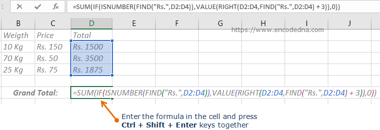
Ok, we got the total cost for each product, by multiplying the cells value in the above example. Now, let’s calculate the Grand Total of the Total.
Here too we are dealing with cells with text and numbers. You cannot use the SUM() function alone to get the grand total, since the values are alphanumeric.
Now, here’s the formula.
=SUM( IF( ISNUMBER( FIND("Rs.",D2:D4)), VALUE( RIGHT(D2:D4, FIND("Rs.",D2:D4) + 3)),0))
Tip: Don’t just hit the Enter key. You must press Ctrl + Shift + Enter keys together. If it didn’t work, set focus on the formula cell, press F2 and then press Ctrl + Shift + Enter keys together.
See the image.
image

Finally, use the CONCATENATE() function to add the Rs. symbol to the result.
=CONCATENATE("Rs. ", SUM(IF(ISNUMBER(FIND("Rs.",D2:D4)),VALUE(RIGHT(D2:D4,FIND("Rs.",D2:D4) + 3)),0)))
You must press Ctrl + Shift + Enter keys together.
Similarly, you can calculate the sum of cells with alphanumeric values using the SUM() function along with the SUBSTITUTE() function. For example,
=SUM( SUBSTITUTE(B2, "Kg", ""), SUBSTITUTE(C2, "Kg ", ""))
Or, use the + sign.
=SUBSTITUTE(B2, "Kg", "") + SUBSTITUTE(C2, "Kg ", "")
