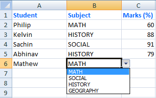
The Dropdown list (in this example) will have a list of pre-defined values from which the user can select the data. This will actually prevent a data entry operator from making mistakes while doing entries in specific cells, since the operator will have to select values the list (it is like a Master data).
The Data Validation option in Excel is ideal for these kind situations. Since it prevents users to entering unnecessary data into the cells. If the data selected in a cell does not match the data in the drop down list, it will throw an error with a message saying the value entered in not valid.
The image that I have attached in the beginning of this article, shows three columns with Students Name, Subject and Marks respectively. The Subject column shows the dropdown control with a list of subjects.
01) Create a new Excel file and open it. By default, it will have three sheets. We need two sheets for the demo. Sheet1 will be used for data entry and Sheet2 will work like a master sheet.
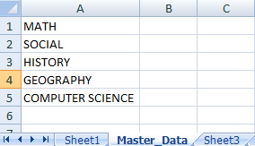
02) Name the sheet2 as Master_Data and add few rows of data in the first column.
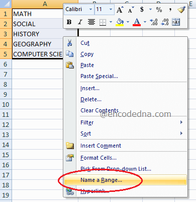
03) Now we need to give these data list a name. Select the rows with master data and right click to choose Name a Range option. This will open the 'New Name' dialog box.
04) In the Name column, type SUBJECTS and do not change the value in Scope column, which is set as Workbook. Now the name range subjects, will be available throughout the workbook.
05) In the same dialog there is another column at the end named Refers to. This will have a range of selections pointing to the “Column” and the number of Rows. For example, we have selected 5 rows in the first column and it read like =Master_Data!$A$1:$A$5.
06) You can reset the range manually if you want to add more data to the list or remove certain values from the list.
Note: Multiple name range can be created and you can have an entire sheet filled with master data. And these lists can be hooked with multiple columns throughout the workbook.
Add the List with the Column
Once you have created the name range it is time to add this range to a column, so that the user can select data from this pre-defined list.
In Sheet1 we have 3 columns as mentioned earlier and the 2nd column named Subject will be hooked to the name range.
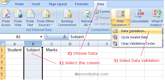
01) Select the column (subject), in which we want to show the dropdown list. From the top menu, click the Data tab and find Data Validation tool. Clicking the button will open the Data Validation dialog box.
02) In Settings tab you will see a list of validation criteria. In the Allow dropdown list, choose the option List. It will now show a input box named Source.
03) The Source will be the master data showing a list of pre-defined values in a dropdown list. In the input box enter =SUBJECTS. This is the name range we created in Sheet2.
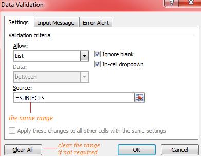
Well, that's it. Now, everytime you set focus on a cell in 2nd column, it will show a Dropdown list with the values from the name range SUBJECT.
Remove DropDown List option in Excel
At any point of time if you want to remove the dropdown list from the entire column then open the Data Validation dialog box (follow step 1 and 2) and click the Clear All button and press Ok.
An entire range of master data can be created with different types of values to create multiple dropdown lists. However, it comes with a small drawback. This process is entirely manual and if the user copies data from another cell or range and pastes it in a cell (or the entire range) with Data Validation, then the validation will not work.
Coping and pasting data in Excel sheets are very common, but one has to be careful when pasting data on these cells. This will negate or remove the Data Validation rules.
